- What is Repeated Measures ANOVA?
- Repeated Measures ANOVA Assumptions
- Quick Data Check
- Running Repeated Measures ANOVA in SPSS
- Interpreting the Output
- Reporting Repeated Measures ANOVA
1. What is Repeated Measures ANOVA?

SPSS repeated measures ANOVA tests if the means of 3 or more metric variables are all equal in some population. If this is true and we inspect a sample from our population, the sample means may differ a little bit. Large sample differences, however, are unlikely; these suggest that the population means weren't equal after all.
The simplest repeated measures ANOVA involves 3 outcome variables, all measured on 1 group of cases (often people). Whatever distinguishes these variables (sometimes just the time of measurement) is the within-subjects factor.
Repeated Measures ANOVA Example
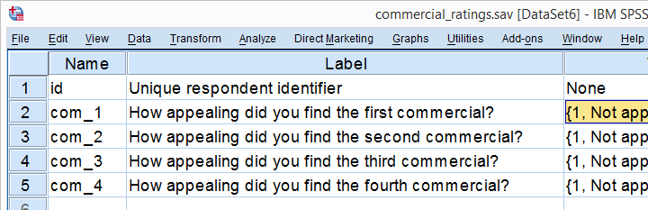
A marketeer wants to launch a new commercial and has four concept versions. She shows the four concepts to 40 participants and asks them to rate each one of them on a 10-point scale, resulting in commercial_ratings.sav.Although such ratings are strictly ordinal variables, we'll treat them as metric variables under the assumption of equal intervals. Part of these data are shown below.
The research question is: which commercial has the highest mean rating? We'll first just inspect the mean ratings in our sample. We'll then try and generalize this sample outcome to our population by testing the null hypothesis that the 4 population mean scores are all equal. We'll reject this if our sample means are very different. Reversely, our sample means being slightly different is a normal sample outcome if population means are all similar.
2. Assumptions Repeated Measures ANOVA
Running a statistical test doesn't always make sense; results reflect reality only insofar as relevant assumptions are met. For a (single factor) repeated measures ANOVA these are
- Independent observations (or, more precisely, independent and identically distributed variables). This is often -not always- satisfied by each case in SPSS representing a different person or other statistical unit.
- The test variables follow a multivariate normal distribution in the population. However, this assumption is not needed if the sample size >= 25.
- Sphericity. This means that the population variances of all possible difference scores (com_1 - com_2, com_1 - com_3 and so on) are equal. Sphericity is tested with Mauchly’s test which is always included in SPSS’ repeated measures ANOVA output so we'll get to that later.
3. Quick Data Check
Before jumping blindly into statistical tests, let's first get a rough idea of what the data look like. Do the frequency distributions look plausible? Are there any system missing values or user missing values that we need to define? For quickly answering such questions, we'll open the data and run histograms with the syntax below.
frequencies com_1 to com_4
/format notable
/histogram.
Result

First off, our histograms look plausible and don't show any weird patterns or extreme values. There's no need to exclude any cases or define user missing values.
Second, since n = 40 for all variables, we don't have any system missing values. In this case, we can proceed with confidence.
4. Run SPSS Repeated Measures ANOVA

 We may freely choose a name for our within-subjects factor. We went with “commercial” because it's the commercial that differs between the four ratings made by each respondent.
 We may also choose a name for our measure: whatever each of the four variables is supposed to reflect. In this case we simply chose “rating”.

 We now select all four variables and move them to the box with the arrow to the right.
Under we'll select .
 Clicking results in the syntax below.
GLM com_1 com_2 com_3 com_4
/WSFACTOR=commercial 4 Polynomial
/MEASURE=rating
/METHOD=SSTYPE(3)
/PRINT=DESCRIPTIVE
/CRITERIA=ALPHA(.05)
/WSDESIGN=commercial.
5. Repeated Measures ANOVA Output - Descriptives
First off, we take a look at the Descriptive Statistics table shown below. Commercial 4 was rated best (m = 6.25). Commercial 1 was rated worst (m = 4.15). Given our 10-point scale, these are large differences.

Repeated Measures ANOVA Output - Mauchly’s Test
We now turn to Mauchly's test for the sphericity assumption. As a rule of thumb, sphericity is assumed if Sig. > 0.05. For our data, Sig. = 0.54 so sphericity is no issue here.

The amount of sphericity is estimated by epsilon (the Greek letter ‘e’ and written as ε). There are different ways for estimating it, including the Greenhouse-Geisser, Huynh-Feldt and lower bound methods. If sphericity is violated, these are used to correct the within-subjects tests as we'll see below.If sphericity is very badly violated, we may report the Multivariate Tests table or abandon repeated measures ANOVA altogether in favor of a Friedman test.
Repeated Measures ANOVA Output - Within-Subjects Effects
Since our data seem spherical, we'll ignore the Greenhouse-Geisser, Huynh-Feldt and lower bound results in the table below. We'll simply interpret the uncorrected results denoted as “Sphericity Assumed”.

The Tests of Within-Subjects Effects is our core output. Because we've just one factor (which commercial was rated), it's pretty simple.
Our p-value, Sig. = .000. So if the means are perfectly equal in the population, there's a 0% chance of finding the differences between the means that we observe in the sample. We therefore reject the null hypothesis of equal means.
The F-value is not really interesting but we'll report it anyway. The same goes for the effect degrees of freedom (df1) and the error degrees of freedom (df2).
6. Reporting the Measures ANOVA Result
When reporting a basic repeated-measures ANOVA, we usually report
- the descriptive statistics table
- the outcome of Mauchly's test and
- the outcome of the within-subjects tests.
When reporting corrected results (Greenhouse-Geisser, Huynh-Feldt or lower bound), indicate which of these corrections you used. We'll cover this in SPSS Repeated Measures ANOVA - Example 2.
Finally, the main F-test is reported as
“The four commercials were not rated equally,
F(3,117) = 15.4, p = .000.”
Thank you for reading!
THIS TUTORIAL HAS 54 COMMENTS:
By Andy Safranski on June 26th, 2015
Excellent tutorial! I was looking for some refresher help on some statistical work and this did the trick. The examples are clear and simple. I really appreciate the end of each tutorial where you lay out the "official way to report".
Thanks much.
By Arthur on July 15th, 2015
Beautiful tutorial!
By Mervin on September 30th, 2015
Hello and thank you for providing this tutorial. If we don't find a significant interaction, do we still have to provide the means?
By Ruben Geert van den Berg on September 30th, 2015
Thanks for your comment! And, indeed, in the absence of an interaction effect, we recommend reporting the main effects (if any). Keep in mind here that small p-values are often not really interesting: they simply say it's highly unlikely that your population effects are zero. Well, if they are not zero, then what's a more plausible indication? The answer is the sample effects, mainly reflected in patterns of means.
So that's a main reason we find the actual means usually more interesting than p-values. Hope that makes some sense.
By Dr. Linus Mhomga on November 3rd, 2015
I found this tutorial helpful and handy as it assisted my understanding of analysis of data by repeated measures ANOVA