- Assumptions for Confidence Intervals for Means
- Any Confidence Level - All Cases
- 95% Confidence Level - Separate Groups
- Any Confidence Level - Separate Groups
- Bonferroni Corrected Confidence Intervals
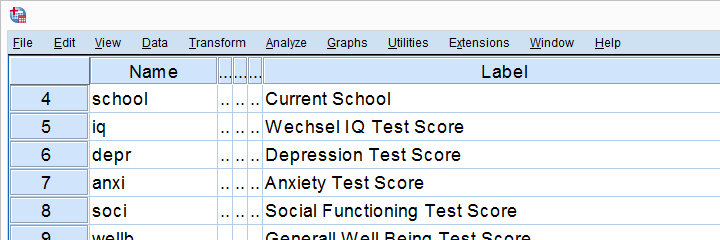
Confidence intervals for means are among the most essential statistics for reporting. Sadly, they're pretty well hidden in SPSS. This tutorial quickly walks you through the best (and worst) options for obtaining them. We'll use adolescents_clean.sav -partly shown below- for all examples.
Assumptions for Confidence Intervals for Means
Computing confidence intervals for means requires
- independent observations and
- normality: our variables must be normally distributed in the population represented by our sample.
1. A visual inspection of our data suggests that each case represents a distinct respondent so it seems safe to assume these are independent observations.
2. Second, the normality assumption is only required for small samples of N < 25 or so. For larger samples, the central limit theorem ensures that the sampling distributions for means, sums and proportions approximate normal distributions. In short,
our example data meet both assumptions.
Any Confidence Level - All Cases I
If we want to analyze all cases as a single group, our best option is the one sample t-test dialog.

The final output will include confidence intervals for the differences between our test value and our sample means. Now, if we use 0 as the test value, these differences will be exactly equal to our sample means.
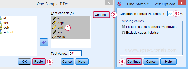
Clicking results in the syntax below. Let's run it.
T-TEST
/TESTVAL=0
/MISSING=ANALYSIS
/VARIABLES=iq depr anxi soci wellb
/CRITERIA=CI(.99).
Result
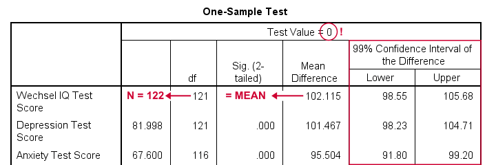
- as long as we use 0 as the test value, mean differences are equal to the actual means. This holds for their confidence intervals as well;
- the table indirectly includes the sample sizes: df = N - 1 and therefore N = df + 1.
Any Confidence Level - All Cases II
An alternative -but worse- option for obtaining these same confidence intervals is from

 We'll discuss these dialogs and their output in a minute under Any Confidence Level - Separate Groups II. They result in the syntax below.
EXAMINE VARIABLES=iq depr anxi soci wellb
/PLOT NONE
/STATISTICS DESCRIPTIVES
/CINTERVAL 95
/MISSING PAIRWISE /*IMPORTANT!*/
/NOTOTAL.
*Minimal syntax - returns 95% CI's by default.
examine iq depr anxi soci wellb
/missing pairwise /*IMPORTANT!*/.
95% Confidence Level - Separate Groups
In many situations, analysts report statistics for separate groups such as male and female respondents. If these statistics include 95% confidence intervals for means, the way to go is the One-Way ANOVA dialog.

Now, sex is a dichotomous variable so we compare these 2 means with a t-test rather than an ANOVA -even though the significance levels are identical for these tests. However, the dialogs below result in a much nicer -and technically correct- descriptives table than the t-test dialogs.
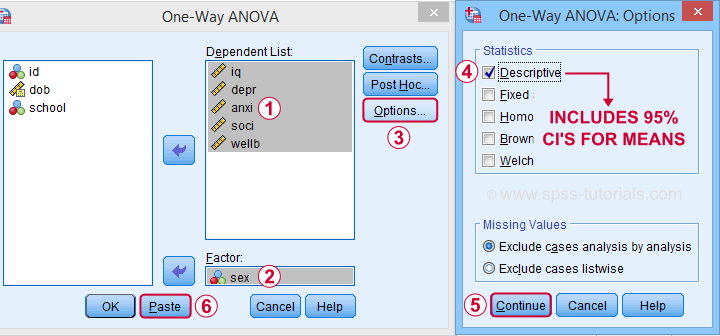
 Descriptives includes 95% CI's for means but other confidence levels aren't available.
 Clicking results in the syntax below. Let's run it.
ONEWAY iq depr anxi soci wellb BY sex
/STATISTICS DESCRIPTIVES .
Result
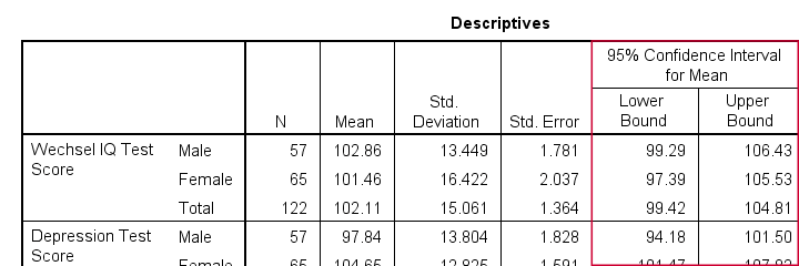
The resulting table has a nice layout that comes pretty close to the APA recommended format. It includes
- sample sizes;
- sample means;
- standard deviations and
- 95% CI's for means.
As mentioned, this method is restricted to 95% CI's. So let's look into 2 alternatives for other confidence levels.
Any Confidence Level - Separate Groups I
So how to obtain other confidence intervals for separate groups? The best option is adding a SPLIT FILE to the One Sample T-Test method. Since we discussed these dialogs and output under Any Confidence Level - All Cases I, we'll now just present the modified syntax.
sort cases by sex.
split file layered by sex.
*Obtain 95% CI's for means of iq to wellb.
T-TEST
/TESTVAL=0
/MISSING=ANALYSIS
/VARIABLES=iq depr anxi soci wellb
/CRITERIA=CI(.95).
*Switch off SPLIT FILE for succeeding output.
split file off.
Any Confidence Level - Separate Groups II
A last option we should mention is the Explore dialog as shown below.

We mostly discuss it for the sake of completeness because
SPSS’ Explore dialog is a real showcase of stupidity
and poor UX design.
Just a few of its shortcomings are that
- you can select “statistics” but not which statistics;
- if you do so, you always get a tsunami of statistics -the vast majority of which you don't want;
- what you probably do want are sample sizes but these are not available;
- the sample sizes that are actually used may be different than you think: in contrast to similar dialogs, Explore uses listwise exclusion of missing values by default;
- what you probably do want, is exclusion of missing values by analysis or variable. This is available but mislabeled “pairwise” exclusion.
- the Explore dialog generates an EXAMINE command so many users think these are 2 separate procedures.
For these reasons, I personally only use Explore for
These tests are under -the very last place you'd expect them.
But anyway, the steps shown below result in confidence intervals for means for males and females separately.
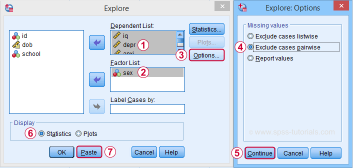
 Clicking generates the syntax below.
EXAMINE VARIABLES=iq depr anxi soci wellb BY sex
/PLOT NONE
/STATISTICS DESCRIPTIVES
/CINTERVAL 95
/MISSING PAIRWISE /*IMPORTANT!*/
/NOTOTAL.
*Minimal syntax - returns 95% CI's by default.
examine iq depr anxi soci wellb by sex
/missing pairwise /*IMPORTANT!*/
/nototal.
Result

Bonferroni Corrected Confidence Intervals
All examples in this tutorial used 5 outcome variables measured on the same sample of respondents. Now, a 95% confidence interval has a 5% chance of not enclosing the population parameter we're after. So for 5 such intervals, there's a (1 - 0.955 =) 0.226 probability that at least one of them is wrong.
Some analysts argue that this problem should be fixed by applying a Bonferroni correction. Some procedures in SPSS have this as an option as shown below.

But what about basic confidence intervals? The easiest way is probably to adjust the confidence levels manually by
$$level_{adj} = 100\% - \frac{100\% - level_{unadj}}{N_i}$$
where \(N_i\) denotes the number of intervals calculated on the same sample. So some Bonferroni adjusted confidence levels are
- 95.00% if you calculate 1 (95%) confidence interval;
- 97.50% if you calculate 2 (95%) confidence intervals;
- 98.33% if you calculate 3 (95%) confidence intervals;
- 98.75% if you calculate 4 (95%) confidence intervals;
- 99.00% if you calculate 5 (95%) confidence intervals;
and so on.
Well, I think that should do. I can't think of anything else I could write on this topic. If you do, please throw us a comment below.
Thanks for reading!
 SPSS TUTORIALS
THIS TUTORIAL HAS 7 COMMENTS:
By Jon K Peck on July 12th, 2023
Custom Tables provides an easy way to do CIs (and other statistics) for the overall sample or separate groups, and you can control the order, significance level and format. You can do this easily with the panel or syntax like this.
CTABLES
/TABLE jobcat BY salary [MEAN.LCL, MEAN, MEAN.UCL]
/CRITERIA CILEVEL=90.
You can also get CIs for the median. And you can have multidimensional subgroups
The ONEWAY procedure does let you set the sig level for the CI in the dialog and in syntax.
EXAMINE is not my favorite procedure by far, but its goal is to give you a let set of measures in one place to help identify interesting things about the distribution. If you already know what characteristics you are interested in rather than exploring, other procedures are a better choice.
By Ruben Geert van den Berg on July 12th, 2023
Hi Jon!
You're right about ONEWAY, the /CRITERIA subcommand (introduced in SPSS 27) does this. I should update my article on this.
P.s. there's an ugly typo in the CSR for SPSS 28 ("The optional CRIERIA subcommand...").