A null hypothesis is a precise statement about a population that we try to reject with sample data. We don't usually believe our null hypothesis (or H0) to be true. However, we need some exact statement as a starting point for statistical significance testing.
Null Hypothesis Examples
Often -but not always- the null hypothesis states there is no association or difference between variables or subpopulations. Like so, some typical null hypotheses are:
- the correlation between frustration and aggression is zero (correlation analysis);
- the average income for men is similar to that for women (independent samples t-test);
- Nationality is (perfectly) unrelated to music preference (chi-square independence test);
- the average population income was equal over 2012 through 2016 (repeated measures ANOVA).
“Null” Does Not Mean “Zero”
A common misunderstanding is that “null” implies “zero”. This is often but not always the case. For example, a null hypothesis may also state that
the correlation between frustration and aggression is 0.5.
No zero involved here and -although somewhat unusual- perfectly valid.
The “null” in “null hypothesis” derives from “nullify”5: the null hypothesis is the statement that we're trying to refute, regardless whether it does (not) specify a zero effect.
Null Hypothesis Testing -How Does It Work?
I want to know if happiness is related to wealth among Dutch people. One approach to find this out is to formulate a null hypothesis. Since “related to” is not precise, we choose the opposite statement as our null hypothesis:
the correlation between wealth and happiness is zero among all Dutch people.
We'll now try to refute this hypothesis in order to demonstrate that happiness and wealth are related all right.
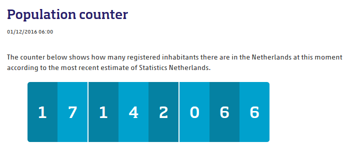
Now, we can't reasonably ask all 17,142,066 Dutch people how happy they generally feel.
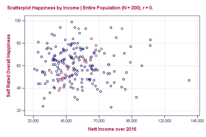
So we'll ask a sample (say, 100 people) about their wealth and their happiness. The correlation between happiness and wealth turns out to be 0.25 in our sample. Now we've one problem: sample outcomes tend to differ somewhat from population outcomes. So if the correlation really is zero in our population, we may find a non zero correlation in our sample. To illustrate this important point, take a look at the scatterplot below. It visualizes a zero correlation between happiness and wealth for an entire population of N = 200.
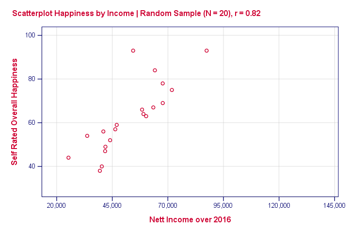
Now we draw a random sample of N = 20 from this population (the red dots in our previous scatterplot). Even though our population correlation is zero, we found a staggering 0.82 correlation in our sample. The figure below illustrates this by omitting all non sampled units from our previous scatterplot.
This raises the question how we can ever say anything about our population if we only have a tiny sample from it. The basic answer: we can rarely say anything with 100% certainty. However, we can say a lot with 99%, 95% or 90% certainty.
Probability
So how does that work? Well, basically, some sample outcomes are highly unlikely given our null hypothesis. Like so, the figure below shows the probabilities for different sample correlations (N = 100) if the population correlation really is zero.
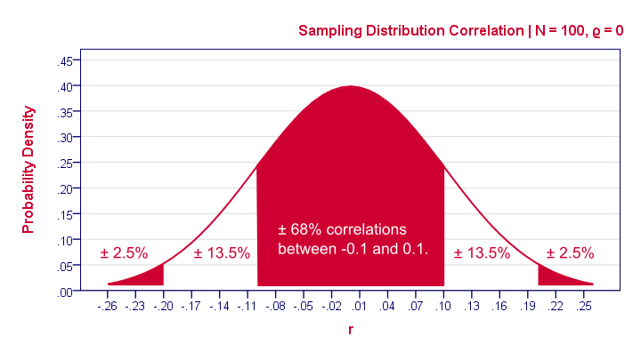
A computer will readily compute these probabilities. However, doing so requires a sample size (100 in our case) and a presumed population correlation ρ (0 in our case). So that's why we need a null hypothesis.
If we look at this sampling distribution carefully, we see that sample correlations around 0 are most likely: there's a 0.68 probability of finding a correlation between -0.1 and 0.1. What does that mean? Well, remember that probabilities can be seen as relative frequencies. So imagine we'd draw 1,000 samples instead of the one we have. This would result in 1,000 correlation coefficients and some 680 of those -a relative frequency of 0.68- would be in the range -0.1 to 0.1. Likewise, there's a 0.95 (or 95%) probability of finding a sample correlation between -0.2 and 0.2.
P-Values
We found a sample correlation of 0.25. How likely is that if the population correlation is zero? The answer is known as the p-value (short for probability value): A p-value is the probability of finding some sample outcome or a more extreme one if the null hypothesis is true. Given our 0.25 correlation, “more extreme” usually means larger than 0.25 or smaller than -0.25. We can't tell from our graph but the underlying table tells us that p ≈ 0.012. If the null hypothesis is true, there's a 1.2% probability of finding our sample correlation.
Conclusion?
If our population correlation really is zero, then we can find a sample correlation of 0.25 in a sample of N = 100. The probability of this happening is only 0.012 so it's very unlikely. A reasonable conclusion is that our population correlation wasn't zero after all.
Conclusion: we reject the null hypothesis. Given our sample outcome, we no longer believe that happiness and wealth are unrelated. However, we still can't state this with certainty.
Null Hypothesis - Limitations
Thus far, we only concluded that the population correlation is probably not zero. That's the only conclusion from our null hypothesis approach and it's not really that interesting.
What we really want to know is the population correlation. Our sample correlation of 0.25 seems a reasonable estimate. We call such a single number a point estimate.
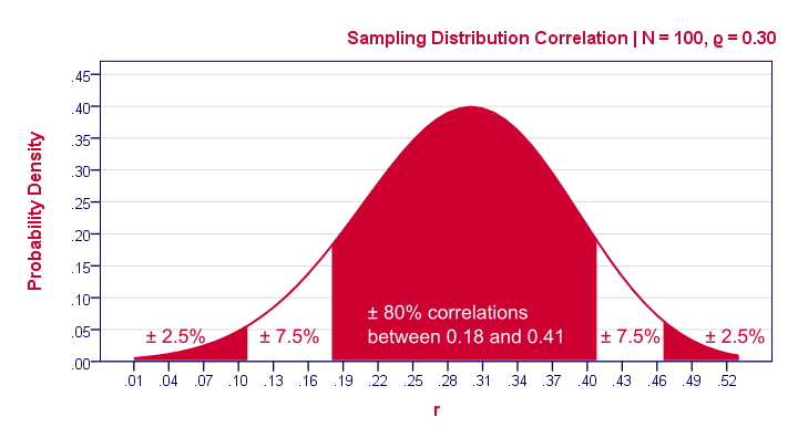
Now, a new sample may come up with a different correlation. An interesting question is how much our sample correlations would fluctuate over samples if we'd draw many of them. The figure below shows precisely that, assuming our sample size of N = 100 and our (point) estimate of 0.25 for the population correlation.
Confidence Intervals
Our sample outcome suggests that some 95% of many samples should come up with a correlation between 0.06 and 0.43. This range is known as a confidence interval. Although not precisely correct, it's most easily thought of as the bandwidth that's likely to enclose the population correlation.
One thing to note is that the confidence interval is quite wide. It almost contains a zero correlation, exactly the null hypothesis we rejected earlier.
Another thing to note is that our sampling distribution and confidence interval are slightly asymmetrical. They are symmetrical for most other statistics (such as means or beta coefficients) but not correlations.
References
- Agresti, A. & Franklin, C. (2014). Statistics. The Art & Science of Learning from Data. Essex: Pearson Education Limited.
- Cohen, J (1988). Statistical Power Analysis for the Social Sciences (2nd. Edition). Hillsdale, New Jersey, Lawrence Erlbaum Associates.
- Field, A. (2013). Discovering Statistics with IBM SPSS Newbury Park, CA: Sage.
- Howell, D.C. (2002). Statistical Methods for Psychology (5th ed.). Pacific Grove CA: Duxbury.
- Van den Brink, W.P. & Koele, P. (2002). Statistiek, deel 3 [Statistics, part 3]. Amsterdam: Boom.
THIS TUTORIAL HAS 17 COMMENTS:
By John Xie on February 28th, 2023
“stop using the term ‘statistically significant’ entirely and moving to a world beyond ‘p < 0.05’”
“…, no p-value can reveal the plausibility, presence, truth, or importance of an association or effect.
Therefore, a label of statistical significance does not mean or imply that an association or effect is highly probable, real, true, or important. Nor does a label of statistical nonsignificance lead to the association or effect being improbable, absent, false, or unimportant.
Yet the dichotomization into ‘significant’ and ‘not significant’ is taken as an imprimatur of authority on these characteristics.” “To be clear, the problem is not that of having only two labels. Results should not be trichotomized, or indeed categorized into any number of groups, based on arbitrary p-value thresholds.
Similarly, we need to stop using confidence intervals as another means of dichotomizing (based, on whether a null value falls within the interval). And, to preclude a reappearance of this problem elsewhere, we must not begin arbitrarily categorizing other statistical measures (such as Bayes factors).”
Quotation from: Ronald L. Wasserstein, Allen L. Schirm & Nicole A. Lazar, Moving to a World Beyond “p<0.05”, The American Statistician(2019), Vol. 73, No. S1, 1-19: Editorial.
By Ruben Geert van den Berg on February 28th, 2023
Yes, partly agreed.
However, most students are still forced to apply null hypothesis testing so why not try to explain to them how it works?
An associated problem is that "significant" has a normal language meaning. Most people seem to confuse "statistically significant" with "real-world significant", which is unfortunate.
By the way, this same point applies to other terms such as "normally distributed". A normal distribution for dice rolls is not a normal but a uniform distribution ;-)
Keep up the good work!
SPSS tutorials