Contents

• Correlation Test - What Is It?
• Null Hypothesis
• Assumptions
• Correlation Test in SPSS
• Reporting

Correlation Test - What Is It?

A (Pearson) correlation is a number between -1 and +1 that indicates to what extent 2 quantitative variables are linearly related. It's best understood by looking at some scatterplots.

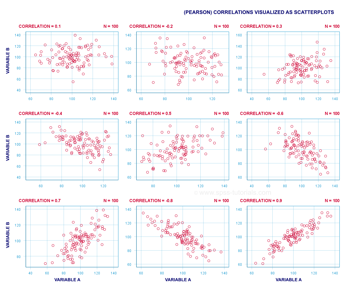
In short,

• a correlation of -1 indicates a perfect linear descending relation: higher scores on one variable imply lower scores on the other variable.
• a correlation of 0 means there's no linear relation between 2 variables whatsoever. However, there may be a (strong) non-linear relation nevertheless.
• a correlation of 1 indicates a perfect ascending linear relation: higher scores on one variable are associated with higher scores on the other variable.

Null Hypothesis

A correlation test (usually) tests the null hypothesis that the population correlation is zero. Data often contain just a sample from a (much) larger population: I surveyed 100 customers (sample) but I'm really interested in all my 100,000 customers (population). Sample outcomes typically differ somewhat from population outcomes. So finding a non zero correlation in my sample does not prove that 2 variables are correlated in my entire population; if the population correlation is really zero, I may easily find a small correlation in my sample. However, finding a strong correlation in this case is very unlikely and suggests that my population correlation wasn't zero after all.

Correlation Test - Assumptions

Computing and interpreting correlation coefficients themselves does not require any assumptions. However, the statistical significance-test for correlations assumes

• independent observations;
• normality: our 2 variables must follow a bivariate normal distribution in our population. This assumption is not needed for sample sizes of N = 25 or more.For reasonable sample sizes, the central limit theorem ensures that the sampling distribution will be normal.

SPSS - Quick Data Check

Let's run some correlation tests in SPSS now. We'll use adolescents.sav, a data file which holds psychological test data on 128 children between 12 and 14 years old. Part of its variable view is shown below.

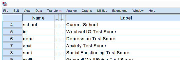
Now, before running any correlations, let's first make sure our data are plausible in the first place. Since all 5 variables are metric, we'll quickly inspect their histograms by running the syntax below.

Histogram Output

Our histograms tell us a lot: our variables have between 5 and 10 missing values. Their means are close to 100 with standard deviations around 15 -which is good because that's how these tests have been calibrated. One thing bothers me, though, and it's shown below.

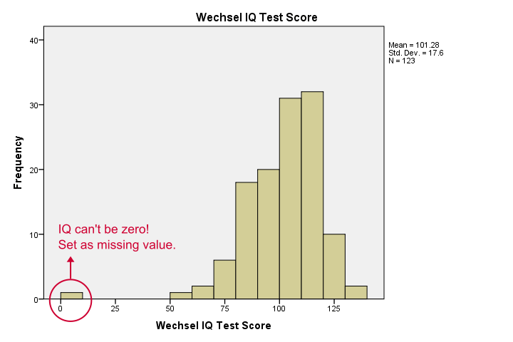
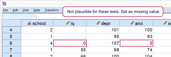
It seems like somebody scored zero on some tests -which is not plausible at all. If we ignore this, our correlations will be severely biased. Let's sort our cases, see what's going on and set some missing values before proceeding.

If we now rerun our histograms, we'll see that all distributions look plausible. Only now should we proceed to running the actual correlations.

Running a Correlation Test in SPSS

Let's first navigate to Analyze Correlate Bivariate as shown below.

Move all relevant variables into the variables box. You probably don't want to change anything else here.

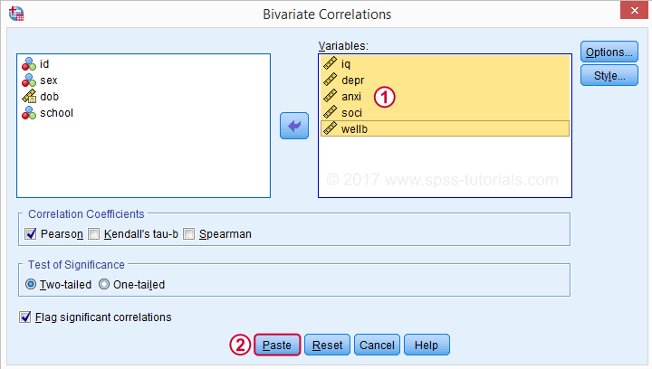
Clicking Paste results in the syntax below. Let's run it.

SPSS CORRELATIONS Syntax

Correlation Output

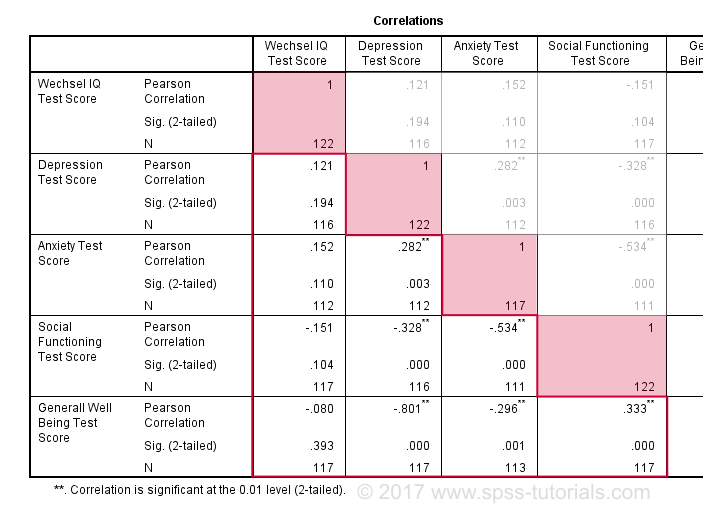
By default, SPSS always creates a full correlation matrix. Each correlation appears twice: above and below the main diagonal. The correlations on the main diagonal are the correlations between each variable and itself -which is why they are all 1 and not interesting at all. The 10 correlations below the diagonal are what we need. As a rule of thumb, a correlation is statistically significant if its “Sig. (2-tailed)” < 0.05. Now let's take a close look at our results: the strongest correlation is between depression and overall well-being : r = -0.801. It's based on N = 117 children and its 2-tailed significance, p = 0.000. This means there's a 0.000 probability of finding this sample correlation -or a larger one- if the actual population correlation is zero.

Note that IQ does not correlate with anything. Its strongest correlation is 0.152 with anxiety but p = 0.11 so it's not statistically significantly different from zero. That is, there's an 0.11 chance of finding it if the population correlation is zero. This correlation is too small to reject the null hypothesis.

Like so, our 10 correlations indicate to which extent each pair of variables are linearly related. Finally, note that each correlation is computed on a slightly different N -ranging from 111 to 117. This is because SPSS uses pairwise deletion of missing values by default for correlations.

Scatterplots

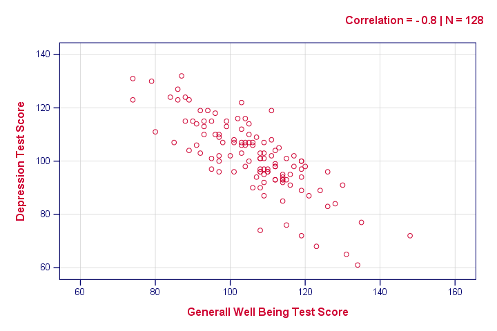
Strictly, we should inspect all scatterplots among our variables as well. After all, variables that don't correlate could still be related in some non-linear fashion. But for more than 5 or 6 variables, the number of possible scatterplots explodes so we often skip inspecting them. However, see SPSS - Create All Scatterplots Tool.
The syntax below creates just one scatterplot, just to get an idea of what our relation looks like. The result doesn't show anything unexpected, though.

Reporting a Correlation Test

The figure below shows the most basic format recommended by the APA for reporting correlations. Importantly, make sure the table indicates which correlations are statistically significant at p < 0.05 and perhaps p < 0.01. Also see SPSS Correlations in APA Format.

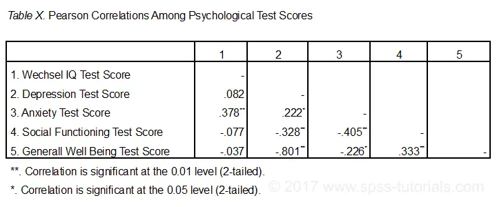
If possible, report the confidence intervals for your correlations as well. Oddly, SPSS doesn't include those. However, see SPSS Confidence Intervals for Correlations Tool.

Thanks for reading!